Geographical Positions from Stellar Azimuths
by Cecil Herman Ney
(Ney, Cecil Herman (1954), Geographical Positions from Stellar Azimuths, Transactions, American Geophysical Union, June 1954, Vol.35, No.3, pp.391-397.)
Abstract : A method is developed whereby latitude, longitude, and azimuth are deduced simultaneously from azimuth observations on three or more stars. The method is particularly advantageous for high latitudes. A set of observation equations of the form x(dφ) + y(dλ) - (dA) + ∫ = 0 are solved by least squares for the best values of (dφ), (dλ) and (dA), the corrections to assumed values of the latitude, longitude, and azimuth. Criteria for sharpness of determination are given. The discussion includes the choice and identification of stars and the computation of a numerical example. Using the most favourable selection of stars, and eliminating personal equation, geographical positions correct, astronomically, to about one half a second of arc may be obtained by this method.
During the last twenty years, two methods have been employed by the Geodetic Survey of Canada for the astronomic determination of position. For Laplace azimuth work, the establishment of provincial boundary lines and the determination of deviations of the vertical, the astronomical telescope oriented in the meridian plane has been used exclusively. For the establishment of stations of second order accuracy for mapping and charting in remote areas of the north, the astrolabe method applied to the precision type theodolite has been employed.
The astrolabe method involves the observation of a number of stars at a fixed altitude in each quadrant of the horizon. To obtain the requisite precision of position determination, rapid changes of star altitude per unit of time are essential. Unfortunately, in polar and subpolar areas, the rate of change of altitude for any particular star is much less than in the more southerly temperate zone. Hence, it is apparent that the astrolabe method is not suitable for work in polar regions.
It is also widely recognized that altitudes cannot be measured with the same degree of precision as horizontal angles. One particularly unfavourable feature inherent to the use of the fixed altitude method is the difficulty of maintaining the theodolite telescope at a fixed vertical angle. For high latitude work, a method of geographical position determination based on the measurement of horizontal angles should, therefore, comprise certain factors of superiority over methods based on the measurement of altitudes.
The method herein proposed for the simultaneous determination of latitude, longitude, and azimuth offers a system based on the movement of stars in azimuth instead of in altitude. It involves the use of differential formulas analogous to those developed by Chauvenet for the determination of latitude, whereby corrections to assumed values of the altitude, latitude, and hour angle are derived from observed altitudes of three or more stars. Under certain conditions, the proposed method may prove of greater utility than the altitude method. Its use would permit the successful completion of an observational program in a remote area, where a damaged vertical circle assembly of a theodolite could not be repaired or replaced. It promises great speed of position determination without the necessity of accurate instrument orientation, and without the preparation of an observing program. In addition, it permits observational work to be carried out when only small parts of the sky are free from clouds. In this respect, it is superior to most other methods.
Generalization of method : As a preliminary step to the observational work, an azimuth reference line is selected on the ground and marked by a suitable target one or two miles distant from the observation station. From an observation on the Sun or a star, or from readings of the magnetic compass, an approximate azimuth AA of the line is assumed. Approximate numerical values φA and λA for the latitude and longitude of the observation station are also assumed. From three independent determinations of the azimuth of the reference line made from three different stars, the corrections of dφ, dλ and dA, to the assumed values of the latitude, longitude, and azimuth are derived algebraically by the use of differential formulas. For a solution of greater accuracy, a series of observations on each of the three selected stars, or observations on a dozen or more different stars, are combined in a least squares solution.
The data used for the calculation of the stars' azimuths Z are the assumed latitude φA, the local sidereal time derived from the differences between Greenwich Sidereal Time and the assumed longitude λA, and the stars' declinations. Where the star observations are restricted to Fundamental Stars, the errors in declination may be assumed to be negligible.
Development of differential formulas : By a differentiation of the fundamental spherical trigonometric formula
sin B cot A = sin c cot a - cos c cos B ……………………………………………….(1)
where A, B, and c are allowed to vary, there may be derived the differential formula
dA = - (sin A cos C/sin B) dB - (sin A cos b/sin dc …………………………………(2)
For the astronomical triangle PZS, where P the pole, Z the zenith, and S the star, replace B, A, and C of the spherical triangle, and where dc = -dφ, and dτ = -dλ
dZ = (15 sin Z cos S/sin τ) dλ + (sin Z/tan ξ) dφ …………………………………….(3)
where Z is the azimuth, τ the hour angle, S the parallactic angle, ξ the zenith distance, δ the declination, φ the latitude, λ the longitude, and where dZ and dφ are in seconds of arc, and dλ in seconds of time.
Equation (3), which may be found in a slightly different form in Volume I of Chauvenet's Spherical and Practical Astronomy, gives the change dZ in the computed azimuth due to the small differences d and dφ between the assumed and true longitudes, and the assumed and true latitudes respectively.
The coefficients (15 sin Z cos S)/(sin τ) and (sin Z)/(tan ξ) may be determined with the aid of graphs. First, calculate the azimuth for each star pointing, and the parallactic angle and zenith distance for the first and last pointing of a series. The values of the cosine of the parallactic angle and the tangent of the zenith distance may then be taken by inspection from a graph constructed to show the rates of change in cos S and tan ξ. For a series of observations over a relatively short time, the curves may be assumed to be linear.
The azimuth Z of the star should be computed from the hour angle formula
tan Z = - (cot δ sec φ sin τ)/(1 - cot δ tan φ cos τ) ……………………………………(4)
For close circumpolars, Table 13 of US Coast and Geodetic Survey Special Publication 237 is helpful.
The parallactic angle S may be deduced from the formula
sin S = cos φ sin Z/cos δ …………………………………………………..………….(5)
The zenith distance may be derived from readings of the vertical circle of the theodolite. However, it is probably more convenient to deduce it from the formula
sin ξ = cos δ sin τ /sin Z ……………………………………………………..………. (6)
In Figure 1, let AO the observed azimuth of the reference line AB be equal to the sum of AA the assumed azimuth, plus the unknown correction dA to be derived in the reduction of the observations.
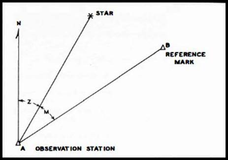
Figure 1 : Measured and computed horizontal angles.
Also, from the observation on the star S, the observed azimuth of the line is equal to Z the computed azimuth of the star, plus dZ the differential change due to the errors dλ and dφ, in the assumed longitude and latitude of the observation station A, plus M the angle measured clockwise from the star to the reference line.
In algebraic form, we have then the two equations
AO = AA + dA …………………………………………………………………….…..(7)
AO = Z + (15 sin Z cos S/sin τ) dλ + (sin Z/tan ξ) dφ + M …………………….……. (8)
Equating (7) and (8), and rearranging, we derive
(sin Z/tan ξ) dφ + (15 cos S sin Z/sin τ) dλ = dA + (Z + M - AA) = 0 ……………….(9)
Conventions : In the measurement of hour angle, azimuth, and parallactic angle, the following conventions must be kept in mind.
The hour angle τ is measured from the local meridian westerly from zero to 360º.
Azimuth is measured from the north clockwise from zero to 360º.
The signs of the coefficients (sin Z/tan ξ) and (15 cos S sin Z)/(sin τ) are usually governed by the signs of sin Z and sin τ. However, for close circumpolar stars, the parallactic angle S may be greater than 90º in which case cos S is a negative quantity.
After the observation of three or more suitably chosen stars, the unknowns dφ, dλ and dA are determined from the solution of a corresponding number of observation equations conforming to the pattern of Equation (9).
The observed values of the desired coordinates and azimuth and found by adding the derived corrections to the assumed values. Hence, we have
φO = φA + dφ, λO = λA + dλ and AO = AA + dA ………………………….………..(10)
Selection of stars for sharp solution : The sharpness of the least squares solution of the observation equations and the accuracy of the final results depend, in large measure, on the suitable choice of stars selected for observation. Where only three stars are observed, they should be so chosen that one of them influences strongly the determination of the latitude, one the longitude, and one the azimuth.
To select a star which will strongly influence the determination of the longitude, it is necessary to know under what conditions the coefficient of dτ in Equation (3) becomes numerically large.
From (3)
dZ = - (sin Z cos S/sin τ) 15 dτ
But
sin Z = sin S cos δ/cos φ
sin τ = sin S sin ξ/cos φ
Substituting these values of sin Z and sin τ, there results
dZ = (cos S cos δ/sin ξ) 15 dτ
For dZ a maximum, both S and ξ must be equal to zero. This occurs when the star is in the meridian and in the zenith. Obviously, it would be impossible to make observations for azimuth when such conditions obtained. The best compromise would be the selection of a southern star within 20º or 30° of the meridian and between 40º and 60° in altitude.
For the special case where the star is observed in the meridian, the parallactic angle becomes zero and
dZ = (cos δ/sin ξ) 15 dτ = (1/A) 15 dr
where A is the azimuth coefficient in the observation equation used in the determination of the clock correction in precise astronomical work by means of the astronomical telescope oriented in the meridian plane. Tabulated values of A, for varying values of δ and ξ as arguments, may be found in US Coast and Geodetic Survey Special Publication 237.
Table 1 gives the approximate values of 15/A for varying values of declination and zenith distance. To select a star which will have a preponderant influence on the determination of the latitude, we again consider Equation (3), where
dZ = (sin Z/tan ξ) dφ
|
Table 1 : Values of 15/A |
||||
|
ξ |
δ |
|||
|
0º |
10º |
15º |
20º |
|
|
30º |
30.00 |
29.40 |
28.95 |
28.20 |
|
35º |
26.25 |
25.95 |
25.35 |
24.60 |
|
40º |
23.40 |
23.10 |
22.35 |
22.05 |
|
45º |
21.15 |
20.85 |
20.55 |
19.95 |
|
Table 2 : Coefficient sin Z/tan ξ |
||||
|
ξ |
Z |
|||
|
90º |
80-100º |
70-110º |
60-120º |
|
|
30º |
1.7 |
1.7 |
1.6 |
1.5 |
|
40º |
1.2 |
1.1 |
1.1 |
1.0 |
|
45º |
1.0 |
1.0 |
0.9 |
0.9 |
|
50º |
0.8 |
- |
- |
- |
In this case, the coefficient sin Z/tan ξ will have a maximum value when Z equals 90º or 270º and when ξ is zero. Here again, azimuth observations would be impossible for a star in the zenith. As the best compromise, a star should be selected which is within 10º or 20º of the prime vertical and between 40º and 60° in elevation. Table 2 shows approximate values of the coefficient for varying values of the azimuth and zenith distance. For a sharp determination of azimuth, a circumpolar star should be observed near elongation. However, in actual practice the choice of any circumpolar star at any hour will give good results.
The identification of stars : The utilization of the azimuth method of position determination necessitates the recognition or easy identification of the stars observed. Most experienced observers are able to recognize the first magnitude stars by sight. As these are the celestial bodies most useful for observation, no difficulty should ensue, except where observations are made through holes in the clouds. As a precautionary measure, it is advisable to read a vertical angle on each star at the time of the first pointing in azimuth. This will obviate any uncertainty of identification when the mathematical reduction is begun.
Knowing the approximate latitude, longitude, altitude, azimuth, and local sidereal time, an unknown star may be easily identified in three or four minutes by having recourse to the following method.
From Equation (6) we have the relationship
cos δ sin τ = sin ξ sin Z or sin τ = sin ξ sin Z/cos δ ……………………. (11)
From simultaneously observed values of ξ and Z, the values of sin ξ sin Z may be computed. Next, an approximation of the star's polar distance is made by noting the star's position in the sky with respect to the pole star.
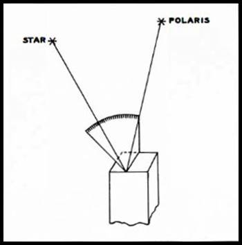
Figure 2 : Star identification.
A more accurate approximation of the polar distance can be made by actual measurement on a cardboard protractor which can be constructed in a few minutes. To secure maximum accuracy in its use, nail a board to the stump of a tree (Figure 2) so that the upper edge is pointing towards Polaris. Place one edge of the cardboard protractor along the edge of the board; rotate the cardboard about this line till the plane of the protractor intersects the star chosen for observation. In this position the protractor lies in the plane defined by the selected star, Polaris and the observer. The polar distance can then be read directly from the graduations.
In carrying out this procedure, it is assumed that Polaris is at the North Pole. The error in the measured polar distance due to the lack of coincidence of Polaris and the Pole will have a maximum value a plus or minus one degree. A correction to the measured value, which may be estimated mentally, may be applied if the added accuracy is required.
The value of τ having been computed from Equation (11), the star's right ascension is derived from the relationship
α = θ – τ
By consulting the publication Apparent Places of Fundamental Stars, the observed star may be identified at once by referring to the tabulated values of the right ascensions and declinations.
Numerical example : To demonstrate the feasibility of the method, a short observational program was carried out on November 13, 1952, at Standards Triangulation Station near the Geodetic Survey Building in Ottawa. High precision work was not attempted as the object of the experiment was to show the feasibility of the method. Due to smoke and water vapor in the atmosphere, only five bright stars were observed, some in very unfavourable positions too close to the horizon. As no reflecting prism was available for use with the instrument, pointings could not be made where the altitude exceeded 45° without introducing an unwarranted amount of physical discomfort.
A 5½ inch precision type Wild theodolite, which had no striding level, was used for making the star observations. To minimise the effect of errors in the observed azimuths arising from unknown inclinations of the horizontal axis of the telescope, a special observing technique was used. On several occasions, this system has proved to be of great value in making azimuth determinations with instruments which are not equipped with striding levels.
After levelling the instrument, the telescope is pointed at the star and the image brought into the field of view. The instrument is then clamped in position so that the moving image will cross the vertical wire of the reticule in one or two minutes. The horizontal plate level is then inspected for any error in centring. Any deviation from the exact centre is corrected by a slight movement of the foot screws. The instant of star transit is recorded electrically on a chronograph by depressing a telegraph key when the star intersects the vertical wire. The horizontal circle is then read and recorded. Next, the instrument is turned clockwise and a pointing made on the reference object which usually is located close to the plane of the horizon.
After reversing the instrument, another rough pointing is made on the star as before and the instrument clamped in such a position that the image is approaching the vertical wire. Before the transit takes place, the foot screws are again readjusted to bring the horizontal plate level bubble to the centre of the vial graduations. After the time of transit and the horizontal circle reading (HCR) are recorded, the instrument is turned counterclockwise and a pointing made on the reference object (RO). If the horizontal plate level of the instrument is of a high degree of sensitivity, this technique will give remarkably good results.
|
Observations for geographical position from Stellar Azimuths |
|||||||||
|
Station - Standards Triangulation Station |
|||||||||
|
Ottawa, November 13, 1953 |
|||||||||
|
|
Object
|
Chronometer Time |
HCR |
Elevation (measured) |
|||||
|
h |
m |
s |
d |
m |
s |
d |
m |
||
|
Star 3
|
Formalhaut
RO (reference object) |
23 |
17 |
54.0 |
185
150 |
10
41 |
25.2
10.2 |
14 |
36 |
|
|
|
|
|
|
|
|
|
|
|
|
Star 2 |
Aldebaran
RO |
29 |
26 |
40.5 |
87
150 |
33
41 |
07.8
04.9 |
20 |
56 |
|
|
|
|
|
|
|
|
|
|
|
|
Star 1 |
Polaris
RO |
0 |
11 |
22.0 |
0
150 |
36
41 |
22.2
45.7 |
46 |
15 |
|
|
|
|
|
|
|
|
|
|
|
|
Star 5 |
B Ursae Minoris
RO |
0 |
04 |
05.0 |
347
150 |
41
41 |
34.0
42.7 |
32 |
58 |
|
|
|
|
|
|
|
|
|
|
|
|
Star 4 |
Altair
RO |
23 |
53 |
45.7 |
255
150 |
08
41 |
52.5
29.0 |
26 |
09 |
|
Mean value of clock correction +14.20s |
|||||||||
Reduction of observations : In the mathematical reduction of the observations, the following assumed values were used
φA = 45° 23’ 30”
λA = 75º 42’ 45” (5h 02m 51.0s)
AA = 150º 40’ 10”
The computations of the azimuths, the parallactic angles, and the coefficients of dφ and dλ are not shown in detail. The resulting values, however, are given in Table 3.
|
Table 3 : Tabulation of data for the formation of observation equations |
||||||||||||||||
|
Star |
τ |
Z |
M |
(Z+M-A) |
S |
ξ |
Dφ Coeff. |
Dλ Coeff. |
||||||||
|
|
d |
m |
s |
d |
m |
s |
d |
m |
s |
sec |
d |
m |
d |
m |
|
|
|
1 |
334 |
59 |
25.5 |
0 |
34 |
58.8 |
150 |
05 |
23.5 |
+ 10.3 |
154 |
34 |
43 |
45 |
+ 0.010 |
+ 0.326 |
|
2 |
283 |
24 |
58.5 |
87 |
32 |
30.7 |
63 |
07 |
57.1 |
+ 17.8 |
47 |
00 |
69 |
04 |
+ 0.382 |
- 10.506 |
|
3 |
5 |
45 |
57.0 |
185 |
09 |
49.3 |
325 |
30 |
45.0 |
+ 24.3 |
4 |
11 |
75 |
24 |
- 0.023 |
-13.401 |
|
4 |
61 |
22 |
45.0 |
255 |
08 |
01.5 |
255 |
32 |
36.5 |
+ 28.0 |
43 |
22 |
63 |
51 |
- 0.481 |
-12.033 |
|
5 |
138 |
23 |
27.0 |
347 |
40 |
16.4 |
183 |
00 |
08.7 |
+ 15.1 |
33 |
45 |
57 |
02 |
- 0.138 |
-4.010 |
The following observation equations may be written down at once from the data given in Table 3
|
1 |
Polaris |
+ 0.010 dφ |
+ 0.326 dλ |
- dA + 10.3 = 0 |
|
2 |
Aldebaran |
+ 0.382 dφ |
- 10.506 dλ |
- dA + 17.8 = 0 |
|
3 |
Formalhaut |
- 0.023 dφ |
- 13.401 dλ |
- dA + 24.3 = 0 |
|
4 |
Altair |
- 0.481 dφ |
- 12.033 dλ |
- dA + 28.0 = 0 |
|
5 |
B Ursae Minoris |
- 0.138 dφ |
- 4.010 dλ |
- dA + 15.1 = 0 |
In making the least squares reduction, the first step is the formation of the normal equations as follows, with a check column on the right hand side:
dφ dλ dA Absolute term Sum
+ 0.3970 + 2.6394 + 0.2500 - 9.2081 - 5.9217
+ 450.9423 + 39.6240 - 909.7683 - 413.5626
+ 5.0000 - 95.5000 - 50.6260
A solution of the normals gives the following values of the corrections and their probable errors :
dφ = +9.7” ± 0.8 dλ = +1.048s ± 0.041 dA = +10.3” ± 0.4
By adding the derived corrections to the assumed values of the latitude, longitude, and azimuth, the observed values are obtained.
|
|
Latitude |
Longitude |
Azimuth |
|
Assumed value |
45° 23’ 30.0” |
5h 02m 51.00s |
150° 40’ 10.0” |
|
Correction |
+9.7” |
+1.05s |
+10.3” |
|
Observed value |
45° 23’ 39.7” |
5h 02m 52.05s (75º 43’ 00.7”) |
150° 40’ 20.3” |
The corresponding astronomic values from precise observations made at the same station are
φ = 45° 23’ 40.3” λ = 75° 42” 56.7” A = 150° 40’ 21.6”
The differences between the observed latitude and longitude and the values previously derived for the same station from precise observations are equivalent to 60 feet in latitude and 288 feet in longitude.
It is desirable to emphasise the fact that most of the stars chosen for observation in the illustrative example are at too low an altitude. Consequently, the coefficients of dφ and dλ have values numerically unsuitable for obtaining results of a high degree of accuracy. By observing 15 or 20 stars at suitable positions in the sky, by using an instrument equipped with a striding level, and by ensuring the correct registration of the times of star pointings by using an electric chronograph, it is expected that geographical positions correct, astronomically, to about one half second of arc, could be obtained.
Geodetic Survey of Canada,
Ottawa, Ontario, Canada.